unit 3.5 - Recurrent neural networks (RNN)
Recurrent neural networks or RNN are used to learn data sequences. They are a neural architecture that has important history and that has been supplanted by Transformers since the year 2017. RNN can still have meaningful application in problems with relatively small context windows.
Examples of data sequences:
letters in words
phonemes in speech
predict the next word, language modeling
stock market prediction
temperature in a location
Types of RNN
There are several types of RNN, depending on the task at hand.
1 to 1: predict a value (temperature) from a single previous value
1 to N: generate a caption for an image
N to N: translate a language to another

The basic RNN cell
Remember that RNN are designed to learn a sequence. As such they need to take an input at each time step, but they also need to “remember” previous input using a “state” variable.
The basic RNN cell is a simple neural network layer with 2 inputs instead of one. In most cases the two inputs are concatenated to form one input. The 2 inputs are:
the data input at time \(t\)
the state at \(t-1\)

RNN cells basically process the two input multiple times with the same weights. They can unroll in time as a linear layer that takes 2 inputs.
This is called “vanilla” RNN.
LSTM
The vanilla RNN network has trouble recalling long past information, as the inputs have to travel through small wights multiple times (see section below “Limitation of RNN and why Transfomers”).
As a results AI researchers developed the Long-Short Term Memory or LSTM cell. The LSTM cell has an input \(x\), an output \(h\) and propagates two signals from cell to cell.
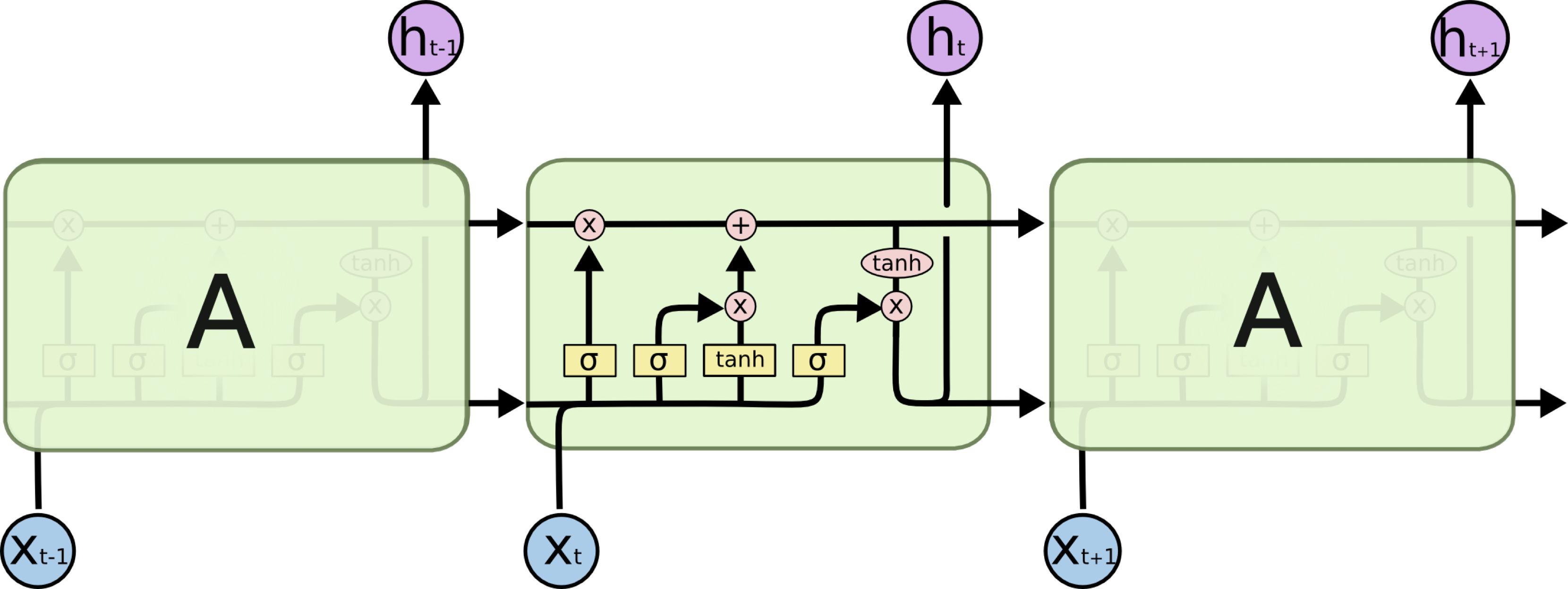
Note the symbols here are:

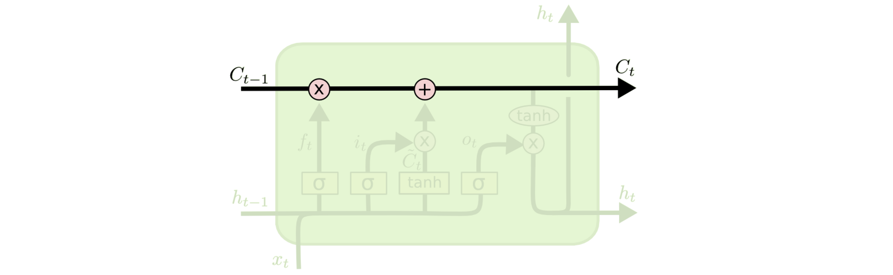
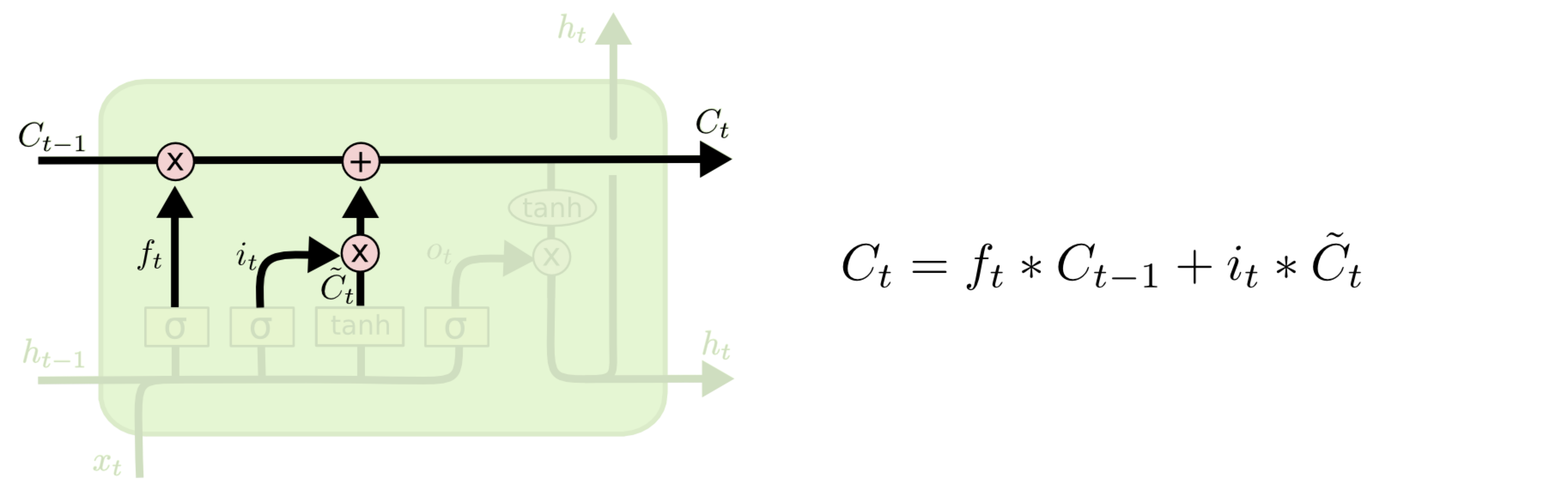
One of the signal that is propagate from cell to cell is the “Cell” state signal \(C\). This signal can be modulated by a weight and information can be added to it. These two modification are applied on the multiplication and addition symbols.
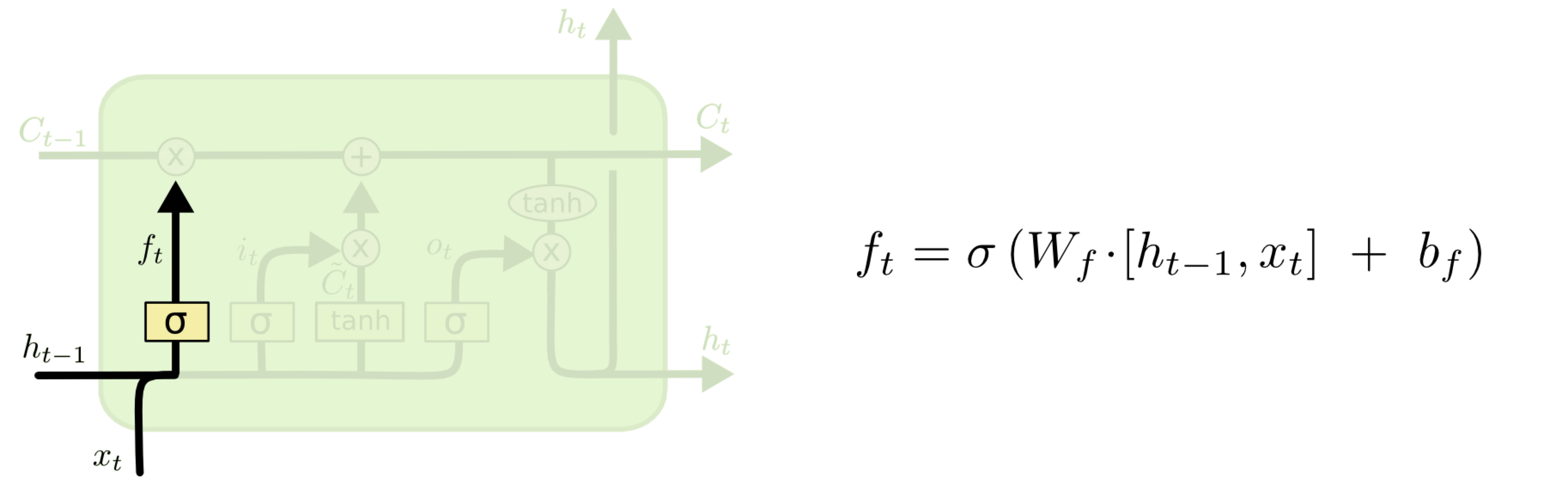
Step 1
Information from the input \(x\) and previous state \(h\) can be processed by a linearl layer called “forget” or \(f\). A sigmoid non-linearity gives the “forget” signal the ability to swing between positive and negative numbers. This signal is what controls how much cell state \(C\) is propagated to the next time-step.
The input \(x\) and previous hidden state \(h\) are used by two more linear layer for processing. One is the “input” \(i\) linear layer, and one if the “new Cell state”.
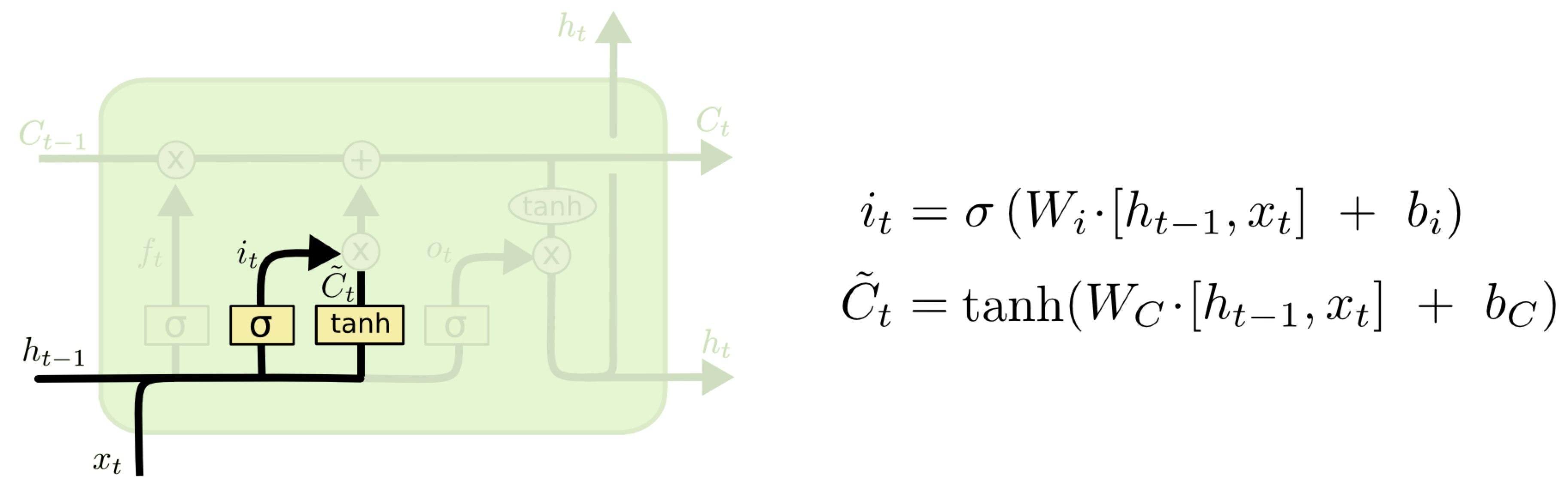
This is how the Cell state is modulated:
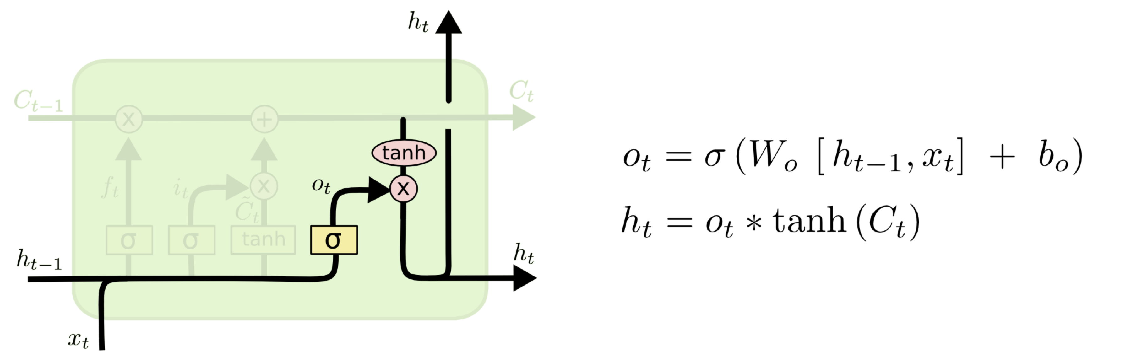
The output \(o\) and stage \(h\) are modulated by another output linear layer:
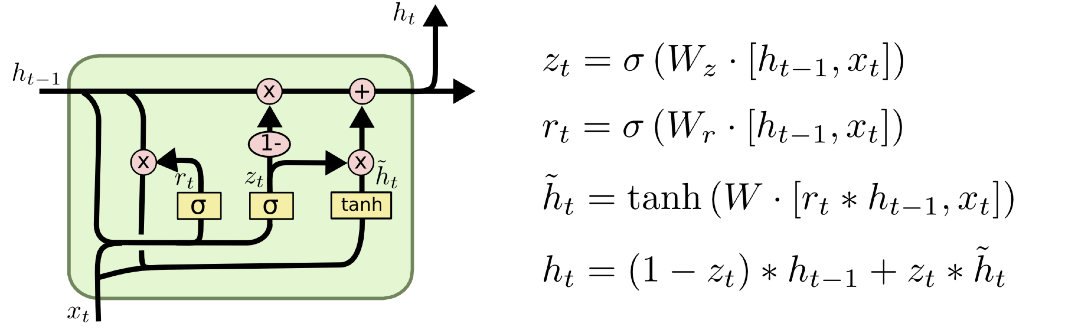
GRU
The Gated-Recurrent-Unit or GRU is a modification of the LSTM cell that uses 4 equations instead of 5 and forgoes one internal state. As such it is slightly more efficient than an LSTM. The improvement is minor, though, and can only be useful in severely resource constrained computational platforms, such as edge computing on micro-controllers.
Note: Some of this material derives from the post (with C. Colah permission).
Limitation of RNN and why Transfomers
Limitation:
cannot remember easily more than ~100 steps in the past
limited by fixed weight
does not build a knowledge graph
Vanishing gradient problem: weights (<1) are multiplied many times by other weights <1: As an example imagine the input goes through 3 weights of 0.1 value: the input after 3 time steps become 0.1 x 0.1 x 0.1 x 0.1 = 0.0001. The inputs are becoming smaller and smaller at each time step, and thus the RNN loses the ability to learn from the past.
Transformer neural networks have proven to be able to create more complex input filters and vast knowledge graphs on inputs. As such they rendered RNN and LSTM virtually obsolete in 2017 with this paper.