unit 0.5 - Approximating functions

Why do we need neural networks? Whate problem do they help solve in a easier way?

Suppose you do a measurement and you get these points:

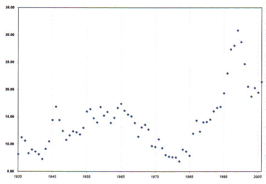
Suppose you want to find the relationship between the independent variable and the dependent ones. What can you do?

Or more in general, if you want to approximate any function or multiple variable, what can you do?

We can start with what we know…

Linear systems

In mathematics, a linear system of equations (or a linear system) is a collection of two or more linear equations involving the same set of variables.

A linear equation is an algebraic equation where each term is either a constant or the product of a constant and a single variable. The variables cannot have exponents (like ), be multiplied together (like ), or be inside functions (like ).

A general system of linear equations with variables () looks like this:

\[\begin{split}\begin{matrix} a_{11}x_1 + a_{12}x_2 + \dots + a_{1n}x_n = b_1 \\ a_{21}x_1 + a_{22}x_2 + \dots + a_{2n}x_n = b_2 \\ \vdots \\ a_{m1}x_1 + a_{m2}x_2 + \dots + a_{mn}x_n = b_m \end{matrix}\end{split}\]

Or in matrix form:

\[\begin{split}\begin{bmatrix} a_{11} & a_{12} & \cdots & a_{1n} \\ a_{21} & a_{22} & \cdots & a_{2n} \\ \vdots & \vdots & \ddots & \vdots \\ a_{m1} & a_{m2} & \cdots & a_{mn} \end{bmatrix} \begin{bmatrix} x_1 \\ x_2 \\ \vdots \\ x_n \end{bmatrix} = \begin{bmatrix} b_1 \\ b_2 \\ \vdots \\ b_m \end{bmatrix}\end{split}\]

When you graph these equations, the visual representation helps explain what a “solution” actually is:

• 2D: Each equation represents a line.

• 3D: Each equation represents a flat plane.

• In higher dimensions: Each equation represents a hyperplane.

Every linear system has exactly one of three possible outcomes:

Outcome	Description	Geometric Meaning
Independent	One unique solution .	The lines/planes intersect at a single point.
Inconsistent	No solution exists.	The lines/planes are parallel and never touch.
Dependent	Infinitely many solutions.	The equations describe the same line/plane (they overlap).

There are several ways to solve these systems depending on their complexity:

• Substitution: Solve one equation for one variable and plug it into the others.

• Elimination: Add or subtract equations to cancel out variables.

• Matrix Algebra: Use an augmented matrix and perform Gaussian Elimination (Row Reduction) to reach “Reduced Row Echelon Form.”

• Cramer’s Rule: Uses determinants (best for small systems).

One issue with this is that it only works for lines or linear functions… but our image above is non linear, what do we do?

Piece-wise linear interpolation

One way to do this is to use piece-wise linear interpolation. We basically divide the range of independent variables into segments, and for each segment we approximate as a line:

\[\begin{split}\hat{f}(x) = \begin{cases} y_0 + \dfrac{y_1 - y_0}{x_1 - x_0}(x - x_0), & x_0 \le x < x_1 \\[8pt] y_1 + \dfrac{y_2 - y_1}{x_2 - x_1}(x - x_1), & x_1 \le x < x_2 \\[8pt] \vdots & \\[4pt] y_{n-1} + \dfrac{y_n - y_{n-1}}{x_n - x_{n-1}}(x - x_{n-1}), & x_{n-1} \le x \le x_n \end{cases}\end{split}\]

Piece-wise linear interpolation is used all the time — neural networks are a very particular, highly scalable version of it. We shall see…

BUT!!!!

1- A piece-wise linear interpolant assumes you already know where the breakpoints (the knots) are. Someone has to decide where x₀, x₁, …, xₙ go. In one dimension that’s manageable. In ten dimensions it’s already painful. In a hundred dimensions it becomes geometrically absurd. The number of regions you’d need to tile the space explodes, and most of them will never see data. Neural networks dodge this by learning the breakpoints instead of hard-coding them. ReLU units are literally learnable kinks: max(0, w·x + b) is a movable hinge in input space.

2- Classical piece-wise linear interpolation also scales badly with dimension because it interpolates on a grid. Grids are innocent in 1D and treacherous in high-D. This is the curse of dimensionality in its purest form: the number of cells grows exponentially with dimension. Neural networks don’t build a grid. They carve the space adaptively, placing linear regions only where the data demands it.

3- Another key difference is generalization. Interpolation is conservative: it behaves nicely between known points but has no opinion outside them. Neural networks are parametric models. They impose a global structure through shared weights, which lets them extrapolate (sometimes badly, sometimes brilliantly) and generalize from sparse data. That weight sharing is a form of inductive bias you don’t get from vanilla interpolation.

4- There’s also an optimization story. Piece-wise linear interpolation is not learned in the usual sense; once the knots are fixed, everything is deterministic. Neural networks turn representation learning into a continuous optimization problem. Gradient descent can slide kinks, rotate hyperplanes, and reconfigure regions smoothly. You’re not searching over combinatorial knot placements; you’re flowing downhill in parameter space.

Polynomial function approximation

We can also use non-linear function approximation, for example we can model any function as an arbitrarily long polynomial.

In polynomial regression, we model the relationship between an independent variable x and a dependent variable y as an n-th degree polynomial. This is the natural bridge between simple linear regression and neural networks because it introduces non-linearity while remaining a linear optimization problem at its core.

\[\hat{y} = w_0 + w_1 x + w_2 x^2 + w_3 x^3 + \cdots + w_d x^d\]

Breakdown of the Components:

y : The predicted output (the “approximation”).

w_0 : The bias or intercept term.

w_1, w_2, … w_d: The learnable weights (coefficients).

x, x^2, x^3 … : The input features, transformed into higher-order powers to allow the model to fit curves rather than just straight lines.

In matrix form:

\[\begin{split}\mathbf{y} = \begin{bmatrix} y_1 \\ y_2 \\ \vdots \\ y_n \end{bmatrix}, \quad \mathbf{X} = \begin{bmatrix} 1 & x_1 & x_1^2 & \cdots & x_1^d \\ 1 & x_2 & x_2^2 & \cdots & x_2^d \\ \vdots & \vdots & \vdots & \ddots & \vdots \\ 1 & x_n & x_n^2 & \cdots & x_n^d \end{bmatrix}, \quad \mathbf{w} = \begin{bmatrix} w_0 \\ w_1 \\ \vdots \\ w_d \end{bmatrix}\end{split}\]

\[\mathbf{y} = \mathbf{X}\mathbf{w}\]

Does this work at scale?

Polynomial regression runs into trouble for essentially the same scaling reasons as piece-wise linear functions. A low-degree polynomial is too rigid: it has global smoothness baked in. If the true function bends sharply in one region and gently in another, the polynomial has to contort everywhere to accommodate that one sharp bend. You get the classic oscillations and edge weirdness. A high-degree polynomial can fit almost anything in 1D, but it pays a price in numerical instability and global coupling: move one data point and the function ripples across the entire domain.

That global coupling is the key limitation. Every coefficient affects the function everywhere. There is no locality. Piece-wise linear models are local: change one knot and only one interval cares. Neural networks sit in between. They are globally parameterized, but locally adaptive. A ReLU network is linear in each region, yet different regions can behave very differently because different subsets of neurons are active.

Dimensionality makes polynomial regression collapse even faster. In multiple dimensions, a degree-d polynomial needs on the order of d^p terms in p dimensions. That combinatorial blow-up is the polynomial version of the curse of dimensionality. You can write it down on paper; you just can’t learn it from finite data. Neural networks again evade the grid by composing low-dimensional nonlinearities. They reuse features across dimensions instead of enumerating all interactions explicitly.

There’s also a bias story. Polynomial regression assumes smoothness of a very specific kind: infinite differentiability and global behavior governed by a single basis. That’s a strong and often wrong prior. Neural networks impose a weaker bias: piece-wise linearity plus compositional structure. That turns out to be a surprisingly good match for many real-world phenomena, which are often smooth-ish locally but stitched together from different regimes.

So yes, the same logic applies, but with a nuance: polynomial regression fails because it is too global and too entangled. Piece-wise linear interpolation fails because it is too local and too brittle. Neural networks work because they land in the narrow middle ground: local behavior with global parameter sharing. That balance is why they scale where the others don’t.