unit 1.7 - Professional training script
![]()
Here we will look at a professional training script in pytorch
You can use this as a REFERENCE for all your projects!
DATASET:
this uses a small dataset used for learning neural networks
[6]:
# PyTorch train script
# https://pytorch.org/tutorials/beginner/basics/optimization_tutorial.html

# We will use the Fashion MNIST dataset: https://www.kaggle.com/datasets/zalando-research/fashionmnist

import torch
from torch import nn
import torch.optim as optim
import torch.nn.functional as F
from torch.utils.data import DataLoader
from torchvision import datasets
from torchvision.transforms import ToTensor

training_data = datasets.FashionMNIST(
    root="data",
    train=True,
    download=True,
    transform=ToTensor()
)

test_data = datasets.FashionMNIST(
    root="data",
    train=False,
    download=True,
    transform=ToTensor()
)
DATA:
If we want to categorize images into classes, we will need a list of possible classes. The output neuros will be the same number as the number of classes.
Before dojg anything else, it is always a good idea to take a look at the data in the dataset!
[7]:
# let us print some data:

categories = ['T-shirt/top', 'Trouser', 'Pullover', 'Dress', 'Coat',
                'Sandal', 'Shirt', 'Sneaker', 'Bag', 'Ankle boot']

# select a random sample from the training set
sample_num = 143
# print(training_data[sample_num])
print('Inputs sample - image size:', training_data[sample_num][0].shape)
print('Label:', training_data[sample_num][1], '\n')

import matplotlib.pyplot as plt

ima = training_data[sample_num][0]
print('Inputs sample - min,max,mean,std:', ima.min().item(), ima.max().item(), ima.mean().item(), ima.std().item())
ima = (ima - ima.mean())/ ima.std()
print('Inputs sample normalized - min,max,mean,std:', ima.min().item(), ima.max().item(), ima.mean().item(), ima.std().item())
iman = ima.permute(1, 2, 0) # needed to be able to plot
plt.imshow(iman)
Inputs sample - image size: torch.Size([1, 28, 28])
Label: 1

Inputs sample - min,max,mean,std: 0.0 1.0 0.28586435317993164 0.392581582069397
Inputs sample normalized - min,max,mean,std: -0.7281654477119446 1.8190758228302002 1.2468318821845514e-08 1.0
[7]:
<matplotlib.image.AxesImage at 0x291b7f590>
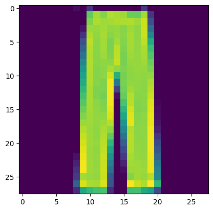
Looks like a pair of pants!
[8]:
class Net(nn.Module):
    def __init__(self):
        super(Net, self).__init__()
        self.flatten = nn.Flatten()
        self.l1 = nn.Linear(28*28, 512)
        self.l2 = nn.Linear(512, 512)
        self.l3 = nn.Linear(512, 10)

    def forward(self, x):
        x = self.flatten(x)
        x = F.relu(self.l1(x))
        x = F.relu(self.l2(x))
        output = self.l3(x)
        return output

# Can also be written as:

# class Net(nn.Module):
#     def __init__(self):
#         super(NeuralNetwork, self).__init__()
#         self.flatten = nn.Flatten()
#         self.linear_relu_stack = nn.Sequential(
#             nn.Linear(28*28, 512),
#             nn.ReLU(),
#             nn.Linear(512, 512),
#             nn.ReLU(),
#             nn.Linear(512, 10),
#         )

#     def forward(self, x):
#         x = self.flatten(x)
#         output = self.linear_relu_stack(x)
#         return output


def train_loop(dataloader, model, loss_fn, optimizer):
    size = len(dataloader.dataset)
    for batch, (X, y) in enumerate(dataloader):
        # Compute prediction and loss
        pred = model(X)
        loss = loss_fn(pred, y)

        # Backpropagation
        optimizer.zero_grad()
        loss.backward()
        optimizer.step()

        if batch % 100 == 0:
            loss, current = loss.item(), (batch + 1) * len(X)
            print(f"loss: {loss:>7f}  [{current:>5d}/{size:>5d}]")


def test_loop(dataloader, model, loss_fn):
    size = len(dataloader.dataset)
    num_batches = len(dataloader)
    test_loss, correct = 0, 0

    with torch.no_grad():
        for X, y in dataloader:
            pred = model(X)
            test_loss += loss_fn(pred, y).item()
            correct += (pred.argmax(1) == y).type(torch.float).sum().item()

    test_loss /= num_batches
    correct /= size
    print(f"Test Error: \n Accuracy: {(100*correct):>0.1f}%, Avg loss: {test_loss:>8f} \n")
Notice our output layer has 10 neurons, just like the number of classes in the dataset.
Let us now train the network
[9]:
# training!

model = Net()

batch_size = 64
train_dataloader = DataLoader(training_data, batch_size=batch_size)
test_dataloader = DataLoader(test_data, batch_size=batch_size)

loss_fn = nn.CrossEntropyLoss() # used for categorization
learning_rate = 1e-3
# note: optimizer is Adam: one of the best optimizers to date
# it can infer learning rate and all hyper-parameters automatically
optimizer = optim.Adam(model.parameters(), lr=learning_rate)

epochs = 10
for t in range(epochs):
    print(f"Epoch {t+1}\n-------------------------------")
    train_loop(train_dataloader, model, loss_fn, optimizer)
    test_loop(test_dataloader, model, loss_fn)
print("Done!")
Epoch 1
-------------------------------
loss: 2.299345  [   64/60000]
loss: 0.571365  [ 6464/60000]
loss: 0.411667  [12864/60000]
loss: 0.506400  [19264/60000]
loss: 0.440894  [25664/60000]
loss: 0.442545  [32064/60000]
loss: 0.380788  [38464/60000]
loss: 0.523417  [44864/60000]
loss: 0.476528  [51264/60000]
loss: 0.513048  [57664/60000]
Test Error:
 Accuracy: 83.4%, Avg loss: 0.439552

Epoch 2
-------------------------------
loss: 0.296889  [   64/60000]
loss: 0.359523  [ 6464/60000]
loss: 0.287938  [12864/60000]
loss: 0.388232  [19264/60000]
loss: 0.377390  [25664/60000]
loss: 0.385652  [32064/60000]
loss: 0.314416  [38464/60000]
loss: 0.529878  [44864/60000]
loss: 0.416916  [51264/60000]
loss: 0.453392  [57664/60000]
Test Error:
 Accuracy: 85.7%, Avg loss: 0.390238

Epoch 3
-------------------------------
loss: 0.223048  [   64/60000]
loss: 0.333038  [ 6464/60000]
loss: 0.229556  [12864/60000]
loss: 0.330350  [19264/60000]
loss: 0.448680  [25664/60000]
loss: 0.359768  [32064/60000]
loss: 0.277115  [38464/60000]
loss: 0.442255  [44864/60000]
loss: 0.326743  [51264/60000]
loss: 0.414322  [57664/60000]
Test Error:
 Accuracy: 86.2%, Avg loss: 0.378768

Epoch 4
-------------------------------
loss: 0.189927  [   64/60000]
loss: 0.306457  [ 6464/60000]
loss: 0.215652  [12864/60000]
loss: 0.290086  [19264/60000]
loss: 0.388842  [25664/60000]
loss: 0.369259  [32064/60000]
loss: 0.241898  [38464/60000]
loss: 0.397346  [44864/60000]
loss: 0.275215  [51264/60000]
loss: 0.327559  [57664/60000]
Test Error:
 Accuracy: 86.8%, Avg loss: 0.355445

Epoch 5
-------------------------------
loss: 0.182914  [   64/60000]
loss: 0.246371  [ 6464/60000]
loss: 0.205581  [12864/60000]
loss: 0.242901  [19264/60000]
loss: 0.413763  [25664/60000]
loss: 0.321556  [32064/60000]
loss: 0.241755  [38464/60000]
loss: 0.402537  [44864/60000]
loss: 0.241768  [51264/60000]
loss: 0.302564  [57664/60000]
Test Error:
 Accuracy: 87.3%, Avg loss: 0.347425

Epoch 6
-------------------------------
loss: 0.195791  [   64/60000]
loss: 0.234772  [ 6464/60000]
loss: 0.166920  [12864/60000]
loss: 0.222736  [19264/60000]
loss: 0.472416  [25664/60000]
loss: 0.304280  [32064/60000]
loss: 0.209779  [38464/60000]
loss: 0.325730  [44864/60000]
loss: 0.265666  [51264/60000]
loss: 0.296183  [57664/60000]
Test Error:
 Accuracy: 88.1%, Avg loss: 0.333879

Epoch 7
-------------------------------
loss: 0.193307  [   64/60000]
loss: 0.188094  [ 6464/60000]
loss: 0.164318  [12864/60000]
loss: 0.242136  [19264/60000]
loss: 0.304813  [25664/60000]
loss: 0.280470  [32064/60000]
loss: 0.204909  [38464/60000]
loss: 0.313631  [44864/60000]
loss: 0.283201  [51264/60000]
loss: 0.260384  [57664/60000]
Test Error:
 Accuracy: 87.7%, Avg loss: 0.349270

Epoch 8
-------------------------------
loss: 0.185134  [   64/60000]
loss: 0.178030  [ 6464/60000]
loss: 0.186955  [12864/60000]
loss: 0.224317  [19264/60000]
loss: 0.263922  [25664/60000]
loss: 0.295104  [32064/60000]
loss: 0.174908  [38464/60000]
loss: 0.330540  [44864/60000]
loss: 0.241252  [51264/60000]
loss: 0.283601  [57664/60000]
Test Error:
 Accuracy: 87.7%, Avg loss: 0.353108

Epoch 9
-------------------------------
loss: 0.149028  [   64/60000]
loss: 0.191820  [ 6464/60000]
loss: 0.167478  [12864/60000]
loss: 0.198771  [19264/60000]
loss: 0.286330  [25664/60000]
loss: 0.239577  [32064/60000]
loss: 0.167874  [38464/60000]
loss: 0.296653  [44864/60000]
loss: 0.224247  [51264/60000]
loss: 0.287964  [57664/60000]
Test Error:
 Accuracy: 87.7%, Avg loss: 0.358775

Epoch 10
-------------------------------
loss: 0.148260  [   64/60000]
loss: 0.138894  [ 6464/60000]
loss: 0.152476  [12864/60000]
loss: 0.188317  [19264/60000]
loss: 0.292156  [25664/60000]
loss: 0.267396  [32064/60000]
loss: 0.193608  [38464/60000]
loss: 0.318536  [44864/60000]
loss: 0.225123  [51264/60000]
loss: 0.240415  [57664/60000]
Test Error:
 Accuracy: 87.2%, Avg loss: 0.388099

Done!
We can now test if the network was trained correctly:
[11]:
sample_num = 143 # select a random sample

with torch.no_grad():
    r = model(training_data[sample_num][0])

print('neural network output pseudo-probabilities:', r)
print('neural network output class number:', torch.argmax(r).item())
print('neural network output, predicted class:', categories[torch.argmax(r).item()])
neural network output pseudo-probabilities: tensor([[-11.9542,  31.1532, -30.3186, -11.9923, -10.9189, -27.4956, -11.2437,
         -48.6321, -12.0049, -27.4024]])
neural network output class number: 1
neural network output, predicted class: Trouser
Important Details
In this script we covered some important details that you may need to study further. Please explore and read the following pages:
The scope of all these topics is quite vast, but at least please read and try to remember the functions and routines you use, and what is available.
Note about the loss function used
In this example we use the cross entropy loss for “categorization tasks”, as in predicting one class out of N
Note about the optimizer used
In this examples we use Adam as an optimizer. Adam is an advanced version of SGD that adjusts hyper-parameters automatically.
HOMEWORK:
Train your neural network with the same architecture for your own data. Get a few images of 3-4 categories of objects from the internet. Resize the images to square size 28x28 just like the example above. You can also modify your network to accept images of different sizes. An example of training data is here. You may want to have a train/ folder and a text/ folder just like in this example here. Train and test data are sets of the same categories of images, but
with different images; train usually has a lot more than test. Use the data loader torchvision.datasets.ImageFolder instead of the torchvision.datasets.FashionMNIST one used above.