unit 1.4 - Back-propagation
![]()
Back-propagation is an optimization algorithm commonly used in training artificial neural networks. It’s a supervised learning algorithm that adjusts the weights of the network to minimize the error between predicted and actual outputs.
Back-propagation is an algorithm that is based on the concept of gradient-descent.
Gradient descent
When we train a neural network we want to minimize the error between the samples from the dataset and the output of the neural networks.
Training a neural network means minimizing the loss function over the dataset.
This is not much different from when you play basketball: you (the neural network) want to get the ball in the basket.

The error function is how much you are off.
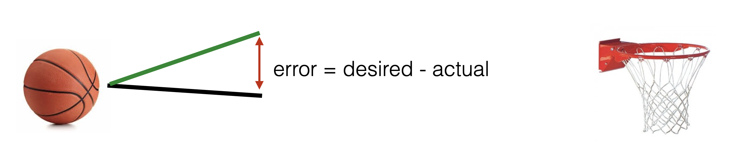
The correction (change in the neural network weights) is how much you have to correct to get the right output (the ball in the basket).

The you just try again…

and again…

until your error is \(~0\) (the ball IS IN the basket!)
This whole process is called “Gradient Descent” and it is the way to find a good set of weights for your neural network that minimizes the loss function.

gradient descent code example
We can now see an example of how this is implemented in python.
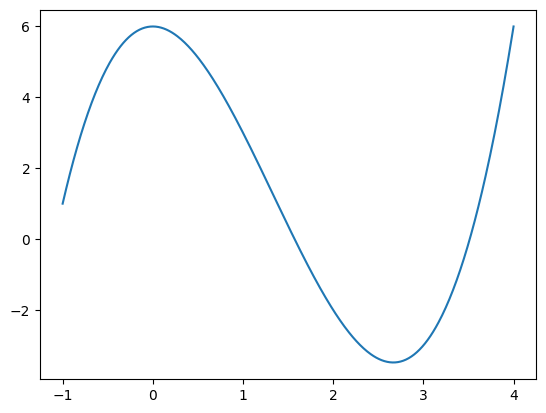
Here is a possible loss function f(x):
\(f(x) = x³-4x²+6\)
[ ]:
import numpy as np
import matplotlib.pyplot as plt

f_x = lambda x: (x**3)-4*(x**2)+6

x = np.linspace(-1,4,500) # plot the curve
plt.plot(x, f_x(x))
plt.show()
Gradient descent is the way we can find the minimum of a function like f(x).
Here is some code implementing gradient descent and an helper function to visualize the algorithm.
[ ]:
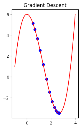
def plot_gradient(x, y, x_vis, y_vis):
plt.subplot(1,2,2)
plt.scatter(x_vis, y_vis, c = "b")
plt.plot(x, f_x(x), c = "r")
plt.title("Gradient Descent")
plt.show()
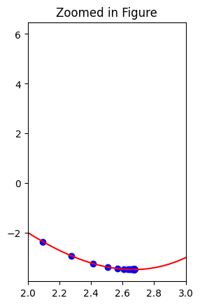
plt.subplot(1,2,1)
plt.scatter(x_vis, y_vis, c = "b")
plt.plot(x,f_x(x), c = "r")
plt.xlim([2.0,3.0])
plt.title("Zoomed in Figure")
plt.show()
def gradient_desc(x_start, steps, learning_rate, delta=0.01):
# These x and y value lists will be used later for visualization.
x_grad = [x_start]
y_grad = [f_x(x_start)]
# Keep looping until number of iterations
for i in range(steps):
# compute the derivative:
x_start_derivative = (f_x(x_start)-f_x(x_start-delta))/delta # derivative approximation
# next point is - learning_rate * derivative:
x_start -= (learning_rate * x_start_derivative)
# update the lists for visualization:
x_grad.append(x_start)
y_grad.append(f_x(x_start))
print ("Local minimum occurs at: {:.2f}".format(x_start))
print ("Number of steps: ",len(x_grad)-1)
plot_gradient(x, f_x(x) ,x_grad, y_grad)
We can now try this on our loss function f(x) and its derivative.
We do this starting at value x = 0.5, using 100 steps, and with a learning-rate of 0.05
[ ]:
gradient_desc(0.5, 100, 0.05)
Local minimum occurs at: 2.67
Number of steps:  100
Note this notebook was inspired by this post.
A numerical example of neural network training
Let’s consider a simple two-layer neural network with two inputs (x1 and x2), two neurons in the first layer (hidden layer), and two neurons in the second layer (output layer). We’ll use a mean squared error (MSE) loss function.
Here’s the architecture:
Inputs: x1, x2
Hidden layer neurons: h1, h2
Output layer neurons: o1, o2

The forward pass can be expressed as follows:
\(h_1 = w_{11} \cdot x_1 + w_{21} \cdot x_2 + b_1\)
\(h_2 = w_{12} \cdot x_1 + w_{22} \cdot x_2 + b_2\)
\(o_1 = w_{31} \cdot h_1 + w_{41} \cdot h_2 + b_3\)
\(o_2 = w_{32} \cdot h_1 + w_{42} \cdot h_2 + b_4\)
Here, \(w\) represents weights, \(b\) represents biases, and the subscripts denote the connection between neurons.
Let’s assume the target outputs are \(y_1\) and \(y_2\). The MSE loss is given by: \(L = \frac{1}{2} \sum_{i=1}^{2} (y_i - o_i)^2\)
Now, we want to minimize this loss using backpropagation.
1. Compute the error terms at the output layer:
$ \delta_{o1} = (o_1 - y_1) \cdot `:nbsphinx-math:sigma`’(o_1)$
$ \delta_{o2} = (o_2 - y_2) \cdot `:nbsphinx-math:sigma`’(o_2)$
Here, \(\sigma'\) is the derivative of the activation function used in the output layer (for simplicity, assume a linear activation, so \(\sigma'(x) = 1\)).
3. Update the weights and biases using the error terms and learning rate (\(\alpha\)):
$ w_{31}^{new} = w_{31} - \alpha `:nbsphinx-math:cdot :nbsphinx-math:delta`_{o1} :nbsphinx-math:`cdot `h_1$
$ w_{41}^{new} = w_{41} - \alpha `:nbsphinx-math:cdot :nbsphinx-math:delta`_{o1} :nbsphinx-math:`cdot `h_2$
$ w_{32}^{new} = w_{32} - \alpha `:nbsphinx-math:cdot :nbsphinx-math:delta`_{o2} :nbsphinx-math:`cdot `h_1$
$ w_{42}^{new} = w_{42} - \alpha `:nbsphinx-math:cdot :nbsphinx-math:delta`_{o2} :nbsphinx-math:`cdot `h_2$
$ w_{11}^{new} = w_{11} - \alpha `:nbsphinx-math:cdot :nbsphinx-math:delta`_{h1} :nbsphinx-math:`cdot `x_1$
$ w_{21}^{new} = w_{21} - \alpha `:nbsphinx-math:cdot :nbsphinx-math:delta`_{h1} :nbsphinx-math:`cdot `x_2$
$ w_{12}^{new} = w_{12} - \alpha `:nbsphinx-math:cdot :nbsphinx-math:delta`_{h2} :nbsphinx-math:`cdot `x_1$
$ w_{22}^{new} = w_{22} - \alpha `:nbsphinx-math:cdot :nbsphinx-math:delta`_{h2} :nbsphinx-math:`cdot `x_2$
4. Update the biases similarly:
$ b_3^{new} = b_3 - \alpha `:nbsphinx-math:cdot :nbsphinx-math:delta`_{o1}$
$ b_4^{new} = b_4 - \alpha `:nbsphinx-math:cdot :nbsphinx-math:delta`_{o2}$
$ b_1^{new} = b_1 - \alpha `:nbsphinx-math:cdot :nbsphinx-math:delta`_{h1}$
$ b_2^{new} = b_2 - \alpha `:nbsphinx-math:cdot :nbsphinx-math:delta`_{h2}$
This process is repeated iteratively until the network converges to a solution that minimizes the error. The learning rate (\(\alpha\)) is a hyperparameter that determines the step size during weight and bias updates. Adjustments may be needed based on the specific problem and dataset.